Lecture 16 – Autoencoders, Sparse Coding, Restricted Boltzmann Machines & Deep Belief Networks

Introduction

Unsupervised Deep Learning plays a critical role in extracting representations from raw data without labels. While supervised networks learn mappings from input to output, unsupervised networks learn the underlying structure and distribution of the data itself. This enables neural networks to compress, denoise, generate, reconstruct, and understand high-dimensional inputs.

In this lecture, we cover the core unsupervised architectures demanded in NCEAC’s official BS Computing Curriculum: Autoencoders, Sparse Autoencoders, Restricted Boltzmann Machines (RBMs), and Deep Belief Networks (DBNs).
These models form the base of modern representation learning, dimensionality reduction, and the early foundations of generative models such as GANs and Variational Autoencoders.

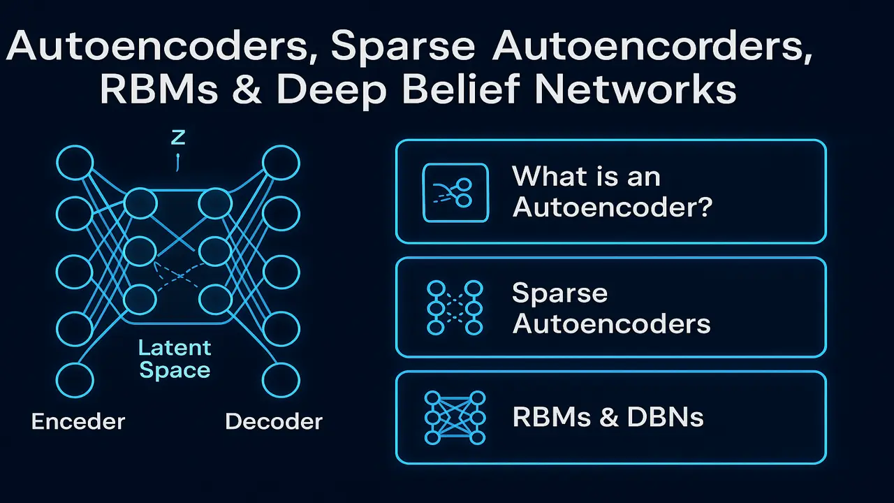
What Are Autoencoders?

Autoencoders are neural networks designed to reconstruct input data.
They consist of two major components:

1. Encoder → compresses the input into a lower-dimensional representation (latent space)
2. Decoder → reconstructs the original input from the latent representation

Mathematically:

z = Encoder(x)
x̂ = Decoder(z)
Loss = ||x – x̂||²

This form of self-supervised learning allows the network to understand meaningful patterns in the data.

Applications:

• Image compression
• Anomaly detection
• Noise removal
• Dimensionality reduction
• Feature extraction
• Data reconstruction
• Pretraining deep models

Autoencoder Architecture (Step-by-Step)

Encoder

Transforms input into compressed code:

x → Dense/Conv Layers → z (latent vector)

The encoder removes redundancy and focuses on essential structure.

Latent Space (The Heart of Autoencoders)

The compressed representation z contains:

• core features
• relationships
• important patterns
• compressed signals

Latent space often captures hidden structure of data.

Decoder

Reconstructs the input from latent vector:

z → Dense/Conv Layers → x̂

The reconstruction error shows how well the model learned the distribution.

Loss Function

Most commonly:

MSE (Mean Squared Error)
Binary Cross Entropy
L1/L2 Loss

Undercomplete vs Overcomplete Autoencoders

Undercomplete AE

• Latent dimension smaller than input
• Forces network to learn meaningful compression
• Best for anomaly detection

Overcomplete AE

• Latent dimension larger than input
• Works only with strong regularization
• Helps learn richer representations

Denoising Autoencoders (DAE)

Denoising AEs learn to recover clean data from corrupted inputs:

Corrupt input → Encoder → Latent → Decoder → Reconstructed Clean Output

Common corruption:

• Gaussian noise
• Salt-and-pepper noise
• Random masking

Applications: Document cleaning, image denoising, MRI restoration, speech enhancement.

Sparse Autoencoders (Required by NCEAC)

Sparse autoencoders impose constraints so that only a small portion of neurons activate at once.

They use:

KL divergence penalty
L1 Regularization
Sparsity constraints on hidden activations

Why Sparse Coding?

Forces network to learn distinctive features
Reduces overfitting
Produces human-interpretable feature maps
Used in medical, image, and text representations

Sparse coding is fundamental to feature extraction and was widely used before deep CNNs.

Lecture 15 – Transformers in Deep Learning: Architecture, Self-Attention, Multi-Head Attention & Positional Encoding

Variants (Stacked Autoencoders, Convolutional Autoencoders)

Stacked Autoencoders

Multiple AEs stacked → deeper latent representations.

Convolutional Autoencoders

Used for:

• Images
• Videos
• Spatial reconstruction

Encoder = Conv layers → Pooling
Decoder = Upsampling → Deconv layers

Restricted Boltzmann Machines (RBMs)

RBM is a two-layer generative stochastic neural network used for unsupervised learning.

RBM consists of:

• Visible layer (v)
• Hidden layer (h)

No intra-layer connections (bipartite graph).
This simplifies computations and makes learning efficient.

Energy Function:

E(v, h) = -aᵀv - bᵀh - vᵀWh

Training method:

Contrastive Divergence (CD-k)

RBMs were crucial for pretraining deep networks before modern methods evolved.

How RBMs Work (Easy Explanation)

Step 1: Initialize visible units with input

Step 2: Compute hidden probabilities

Step 3: Reconstruct visible layer

Step 4: Update weights based on difference

Step 5: Repeat for many epochs

RBMs learn probability distributions over inputs.

Applications of RBMs

Collaborative filtering
Topic modeling
Anomaly detection
Dimensionality reduction
Pretraining DBNs

https://scikit-learn.org

Deep Belief Networks (DBNs)

DBNs are hierarchical deep generative models built by stacking RBMs.

Architecture:

RBM1 → RBM2 → RBM3 → Classifier / Regressor

DBNs are trained layer-wise:

Phase 1 – Pretraining (Unsupervised)

Each RBM learns features from previous RBM.

Phase 2 – Fine-tuning (Supervised)

Final layers trained using backpropagation.

DBNs played a critical role in early deep learning breakthroughs and paved the way for modern architectures.

Autoencoders vs RBMs vs DBNs

Feature	Autoencoders	RBMs	DBNs
Type	Deterministic	Stochastic	Stacked RBMs
Training	Backprop	Contrastive Divergence	Layer-wise
Output	Reconstruction	Probability	Hierarchical features
Use	Feature learning	Generative modeling	Deep representation

Real-World Applications

Medical image denoising
Natural image compression
Fraud detection
Recommendation systems (RBM)
Industrial anomaly detection
OCR & document cleanup
Motion data modeling
Cybersecurity anomaly detection

Performance Analysis

How to evaluate:

Reconstruction Loss

Measures how accurately input is reconstructed.

Latent Space Visualization

t-SNE projections to study structure.

Sparsity Metrics

For sparse AEs.

Sampling Quality

For RBM and DBN outputs.

Coding Perspective

A student must be able to:

Build AE in PyTorch/TensorFlow
Add sparsity regularization
Train RBM using CD-k
Stack RBMs into DBNs
Visualize latent representations
Evaluate reconstruction metrics

Summary

Autoencoders, RBMs, and DBNs form the foundation of classical unsupervised deep learning. They enable networks to learn hidden patterns, compress information, identify anomalies, and generate data without requiring labels. These architectures also paved the way for deep generative models like GANs and Variational Autoencoders, which you will study in Lecture 17.

People also ask: