Lecture 5 – Hidden Markov Models and POS Tagging in Natural Language Processing

Many Natural Language Processing tasks can be described as sequence labelling. There is an input sequence of words and for every word we want to predict a label. Part of speech tagging is one of the most important examples. For every word in a sentence we want to assign a grammatical category such as noun, verb, adjective or preposition. These tags become useful features for syntactic parsing, information extraction and many other tasks.

Hidden Markov Models provide a classical probabilistic framework for sequence labelling. They combine two kinds of information. how likely particular tag sequences are and how likely particular words are for each tag. In this lecture we build intuition for Markov models, define Hidden Markov Models, show how they are used for part of speech tagging and work through the Viterbi algorithm for decoding.

From Tagging Problem to Sequence Model

The input to a part of speech tagger is a sentence such as.

“Students love learning Natural Language Processing.”

The output is a sequence of tags of the same length. For example.

Students. NNS
love. VBP
learning. VBG
Natural. NNP or JJ depending on scheme
Language. NNP
Processing. NNP

The challenge is that many words are ambiguous. The word “race” can be a noun or a verb. The word “book” can be a noun or a verb. The correct tag depends on context.

Two kinds of evidence help.

1. The relation between tags and words. For example, the verb tag is likely for words like “run” and “eat”.
2. The relation between neighbouring tags. For example, a determiner is often followed by an adjective or a noun, not by a verb.

A good sequence model should capture both types of information. Hidden Markov Models do this elegantly.

Markov Chains Recap

Before introducing Hidden Markov Models it is helpful to recall a simpler structure. a Markov chain.

A Markov chain consists of.

1. A set of states.
2. Transition probabilities between states.
3. An initial state distribution.

The key Markov assumption is that the next state depends only on the current state, not on the full history. In other words.

P of state at time t depends on state at time t minus one.

An everyday example is a simple weather model with states “sunny” and “rainy”. There is a certain probability of going from sunny to sunny, sunny to rainy and so on. Given the current weather, we can estimate the probability of different weather sequences.

However, in a Markov chain the states are directly observable. In part of speech tagging the tags are hidden and the words are observed. This leads to the Hidden Markov Model.

Hidden Markov Model Definition

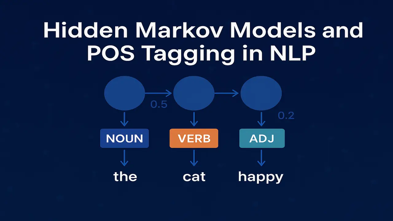
A Hidden Markov Model adds a separate sequence of observations on top of the hidden state sequence. Formally, an HMM consists of.

1. A set of hidden states. In POS tagging these are the part of speech tags.
2. A set of possible observations. These are the words in the vocabulary.
3. Transition probabilities. aij equals the probability of moving from hidden state i to hidden state j.
4. Emission probabilities. bj of w equals the probability of emitting word w when the current hidden state is j.
5. An initial distribution over states at the beginning of the sequence.

During tagging we see only the words. The tags corresponding to the states are hidden. Our job is to infer the most likely state sequence that could have generated the observed word sequence.

The independence assumptions are.

1. The current tag depends only on the previous tag.
2. The current word depends only on the current tag.

These assumptions are approximations, but they make the model tractable and surprisingly powerful.

Applying HMMs to Part of Speech Tagging

To apply an HMM to POS tagging we map directly.

1. Hidden states become POS tags such as Noun, Verb, Adjective, Preposition and so on.
2. Observations become words in the sentence.

Transition probabilities capture patterns like.

1. P of Noun given Determiner is high because determiners are often followed by nouns.
2. P of Verb given Determiner is lower but still possible when there is a gerund form.

Emission probabilities capture how strongly particular words are associated with particular tags. For example.

1. P of “run” given Verb is much higher than P of “run” given Adjective.
2. P of “book” is non zero for both Noun and Verb, reflecting its ambiguity.

For a sentence of words w1 to wN and a candidate tag sequence t1 to tN the joint probability under the HMM is.

P of t1 to tN and w1 to wN equals.

P of t1 times P of w1 given t1 times the product from i equals 2 to N of P of ti given ti minus 1 times P of wi given ti.

The best tag sequence is the one that maximises this joint probability.

Decoding with the Viterbi Algorithm

A naive way to find the best tag sequence would be to enumerate all possible tag sequences and compute their probability. For a sentence of length N and T possible tags this would require T to the power N sequences, which is impossible for realistic values.

The Viterbi algorithm solves this problem efficiently using dynamic programming.

The key observation is that the best path to a given state at position i can be computed from the best paths to all states at position i minus 1, without revisiting complete histories.

For each position i and each tag s we compute.

V at i, s equals the probability of the most likely tag sequence that ends in tag s at position i while generating the first i words.

V at i, s equals the emission probability of the i th word from tag s multiplied by the maximum over previous tags s prime of V at i minus 1, s prime multiplied by the transition probability from s prime to s.

At the same time we store back pointers that remember which previous tag gave the maximum value. After filling the table up to position N we choose the tag with the highest V at N, s and backtrack to recover the entire best sequence.

This yields the most probable tag sequence in time proportional to N times T squared, which is practical for typical tag sets.

Lecture 4 – Language Modeling in Natural Language Processing

Step by step Viterbi Example

Consider a toy tag set with just two tags. Noun and Verb. Suppose we want to tag the two word sentence “fish swim”.

Our HMM has.

1. Initial probabilities. P of Noun is 0 point 6 and P of Verb is 0 point 4.
2. Transition probabilities. P of Noun given Noun is 0 point 3. P of Verb given Noun is 0 point 7. P of Noun given Verb is 0 point 8. P of Verb given Verb is 0 point 2.
3. Emission probabilities. P of “fish” given Noun is 0 point 5. P of “fish” given Verb is 0 point 4. P of “swim” given Verb is 0 point 6. P of “swim” given Noun is 0 point 1.

Step 1. First word “fish”.

V at 1, Noun equals initial Noun times emission of “fish” from Noun, which is 0 point 6 multiplied by 0 point 5 equals 0 point 3.

V at 1, Verb equals initial Verb times emission of “fish” from Verb, which is 0 point 4 multiplied by 0 point 4 equals 0 point 16.

Step 2. Second word “swim”. For each tag we consider both previous tags.

V at 2, Noun equals emission of “swim” from Noun multiplied by the maximum of.

1. V at 1, Noun times transition Noun to Noun equals 0 point 3 times 0 point 3 equals 0 point 09.
2. V at 1, Verb times transition Verb to Noun equals 0 point 16 times 0 point 8 equals 0 point 128.

The maximum is 0 point 128. Multiplying by emission 0 point 1 gives V at 2, Noun equals 0 point 0128.

V at 2, Verb equals emission of “swim” from Verb multiplied by the maximum of.

1. V at 1, Noun times transition Noun to Verb equals 0 point 3 times 0 point 7 equals 0 point 21.
2. V at 1, Verb times transition Verb to Verb equals 0 point 16 times 0 point 2 equals 0 point 032.

The maximum is 0 point 21. Multiplying by emission 0 point 6 gives V at 2, Verb equals 0 point 126.

Since V at 2, Verb is larger than V at 2, Noun the best final tag is Verb. Tracing back through the pointers we find that the best sequence is Noun Verb, which matches our intuition. “fish” is tagged as a noun and “swim” as a verb.

Walking students through such a complete example on a small tag set makes the abstract Viterbi formula intuitive.

Training HMM taggers from corpora

For supervised training we assume access to a tagged corpus where every word already has the correct part of speech tag. This is true for resources such as the Penn Treebank and many modern tagged corpora.

Parameter estimation then becomes simple counting.

1. To estimate transition probabilities we count how often each tag is followed by another tag. P of t2 given t1 equals count of bigram t1 t2 divided by count of t1.
2. To estimate emission probabilities we count how often a word is tagged with a given tag. P of word w given tag t equals count of w tagged as t divided by total count of tag t.
3. To estimate initial probabilities we count how often each tag appears at the beginning of a sentence.

Because the vocabulary is large, many word–tag pairs may be unseen in the training corpus. Smoothing is therefore useful for emission probabilities, just as it was for language models in the previous lecture. A common trick is to replace rare words with a special unknown token and learn its emission probabilities from a separate set of sentences.

Unsupervised training is also possible using the Baum–Welch algorithm, which is a form of expectation maximisation, but this is more advanced and usually not required in an introductory course.

For a full theoretical treatment of POS tagging and HMM taggers, see the POS tagging chapter in Speech and Language Processing.

Real World Examples and Limitations

Hidden Markov Models were the dominant method for POS tagging and other sequence labelling tasks for many years. High quality HMM taggers achieved accuracies around ninety six to ninety seven percent on English newswire text when trained on large corpora.

Examples of real world usage include.

1. Classical taggers implemented in toolkits such as NLTK and in many legacy NLP pipelines.
2. Taggers for morphologically rich languages, where tags incorporate case, gender and number information and where sequence information is extremely helpful.
3. Other sequence tasks that can be framed as tagging, such as named entity recognition or shallow chunking, when implemented as HMMs.

However, HMM taggers have some limitations.

1. They are based on relatively simple independence assumptions that ignore long distance context.
2. They handle rich feature sets less naturally than discriminative models such as Conditional Random Fields.
3. Modern neural models, including recurrent networks and transformers, usually give higher accuracy when sufficient data and compute are available.

Despite these limitations, HMMs remain an essential teaching tool because they make the relationship between probability theory and sequence labelling completely transparent.

Python code example. tiny HMM POS tagger

The following example shows a very small HMM style tagger implemented with simple dictionaries. It is not industrial strength but it clearly demonstrates the Viterbi idea.

import math
from collections import defaultdict

# Toy tagged corpus
tagged_sentences = [
    [("the", "DET"), ("dog", "N"), ("barks", "V")],
    [("the", "DET"), ("cat", "N"), ("meows", "V")],
    [("a", "DET"), ("dog", "N"), ("runs", "V")],
]

# Estimate transition and emission probabilities with add-one smoothing
tags = set()
transition_counts = defaultdict(lambda: defaultdict(int))
emission_counts = defaultdict(lambda: defaultdict(int))
start_counts = defaultdict(int)

for sent in tagged_sentences:
    prev_tag = "<START>"
    start_counts[sent[0][1]] += 1
    for word, tag in sent:
        tags.add(tag)
        transition_counts[prev_tag][tag] += 1
        emission_counts[tag][word] += 1
        prev_tag = tag
    transition_counts[prev_tag]["<END>"] += 1

V = len({w for s in tagged_sentences for (w, _) in s})
T = len(tags)

def log_prob_transition(prev_tag, tag):
    num = transition_counts[prev_tag][tag] + 1
    denom = sum(transition_counts[prev_tag].values()) + (T + 1)
    return math.log(num / denom)

def log_prob_emission(tag, word):
    num = emission_counts[tag][word] + 1
    denom = sum(emission_counts[tag].values()) + V
    return math.log(num / denom)

def viterbi(words):
    dp = []
    back = []
    # initialise
    first_col = {}
    back_first = {}
    for tag in tags:
        lp = log_prob_transition("<START>", tag) + log_prob_emission(tag, words[0])
        first_col[tag] = lp
        back_first[tag] = None
    dp.append(first_col)
    back.append(back_first)

    # recursion
    for i in range(1, len(words)):
        col = {}
        back_col = {}
        for tag in tags:
            best_score = -1e9
            best_prev = None
            for prev_tag in tags:
                score = (
                    dp[i-1][prev_tag]
                    + log_prob_transition(prev_tag, tag)
                    + log_prob_emission(tag, words[i])
                )
                if score > best_score:
                    best_score = score
                    best_prev = prev_tag
            col[tag] = best_score
            back_col[tag] = best_prev
        dp.append(col)
        back.append(back_col)

    # termination
    best_final = None
    best_score = -1e9
    for tag in tags:
        score = dp[-1][tag] + log_prob_transition(tag, "<END>")
        if score > best_score:
            best_score = score
            best_final = tag

    # backtrack
    tags_out = [best_final]
    for i in range(len(words) - 1, 0, -1):
        tags_out.append(back[i][tags_out[-1]])
    tags_out.reverse()
    return list(zip(words, tags_out))

print(viterbi(["the", "dog", "runs"]))

When run, this code outputs a tagged version of the input sentence, demonstrating how transition and emission probabilities combine to choose tags. Students can modify the small corpus and observe how the tagger behaviour changes.

Step by step Algorithm Explanation

The Viterbi decoding process for HMM POS tagging can be summarised as follows.

Step 1. Precompute transition and emission probabilities from a tagged corpus.

Step 2. For a new sentence, create a table with one column per word and one row per tag.

Step 3. Initialise the first column using initial state probabilities multiplied by emission probabilities for the first word.

Step 4. For each later position i and each candidate tag, compute the maximum over previous tags of the probability of the best path to that previous tag multiplied by the transition probability to the current tag, then multiplied by the emission probability of the current word from that tag. Store this value and remember which previous tag achieved the maximum.

Step 5. After filling the last column, select the tag with the highest value as the final tag.

Step 6. Follow back pointers from the last column to the first to recover the entire best tag sequence.

This algorithm ensures that every possible tag sequence is implicitly considered but without enumerating them explicitly.

Summary

Hidden Markov Models provide a clean probabilistic framework for part of speech tagging and other sequence labelling tasks. By modelling both transitions between tags and emissions of words from tags, they combine contextual and lexical information in a principled way. The Viterbi algorithm makes it practical to decode the most likely tag sequence, and simple counting methods allow parameters to be estimated from tagged corpora.

Although more recent neural architectures often achieve higher accuracy and can incorporate richer features, the HMM approach remains foundational. It demonstrates how Markov assumptions, probability distributions and dynamic programming come together to solve a core NLP problem. Understanding HMM tagging prepares students to appreciate more advanced sequence models such as Conditional Random Fields and recurrent or transformer based neural networks.

Next. Lecture 6 – Deterministic and Stochastic Grammars, CFGs and Parsing in NLP.

People also ask: