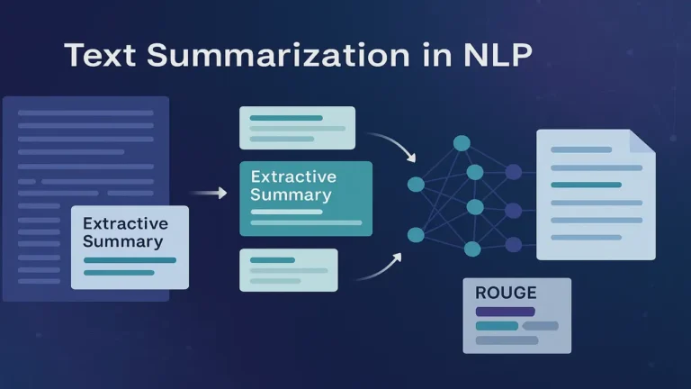
Lecture 11 - Information Retrieval, Vector Space Model and Evaluation

Understand information retrieval basics, vector space model, cosine similarity and evaluation using precision and recall.

Search is one of the most visible applications of Natural Language Processing. Whenever a user types “best deep learning tutorials”, “POS tagging example in Python” or “NLP notes” into a search box, an information retrieval system decides which documents to show and in what order. This lecture explains how information retrieval relates to NLP and search engines, introduces the vector space model with cosine similarity, and covers evaluation using precision, recall and F1.

The goal is to connect your earlier understanding of corpora, bag-of-words and TF-IDF with the way real search engines index, represent and rank documents.

Information retrieval, NLP and search engines

Information retrieval focuses on finding relevant documents from a large collection in response to a user query. NLP provides tools for understanding and representing language. Search engines are large systems that bring these ideas together with additional engineering and ranking signals.

Information retrieval answers questions such as.

What is the best way to represent a document mathematically so that its content can be compared with a query
How should we rank documents so that the most relevant ones appear at the top of the results list
How do we measure whether a retrieval system is performing well or not

Natural Language Processing supports information retrieval by improving tokenisation, handling multiple languages, normalising word forms, detecting phrases, recognising spelling errors and sometimes using semantic representations instead of just surface words.

A search engine is more than just IR and NLP. It also includes crawling, indexing at web scale, dealing with duplicate content, exploiting user click signals, personalised ranking and many other components. In this lecture, we focus on the core IR part that any NLP student should understand.

Indexing basics

If we have a small collection of ten short documents, we could scan all of them for every query and still return answers quickly. But real systems deal with millions or billions of documents. Linear scanning would be far too slow. To support fast retrieval, systems build an inverted index.

The inverted index is similar to the index at the back of a book but built automatically. Instead of mapping topics to page numbers, we map terms to lists of documents.

Indexing pipeline.

Document collection. Define the corpus. this could be web pages, lecture notes, research articles, product descriptions or support tickets.
Text preprocessing. Apply the steps you saw earlier. lowercasing, tokenisation, optional stopword removal, maybe stemming or lemmatisation.
Vocabulary creation. Extract the set of distinct terms that appear in the corpus, often ignoring extremely rare tokens.
Inverted index construction. For each term, store a posting list of all documents that contain that term, often with additional information such as term frequency or positions within the document.

For example, suppose we have documents d1 to d5. After preprocessing, the index might contain entries like.

“vector” → [d2, d4, d5]
“retrieval” → [d1, d3, d5]
“cosine” → [d4, d5]

When a user query includes the word “retrieval”, the system can jump directly to the posting list for “retrieval” instead of scanning all documents. Combining posting lists for all query terms quickly gives a set of candidate documents that will then be scored and ranked.

This inverted index is at the heart of almost every production search system.

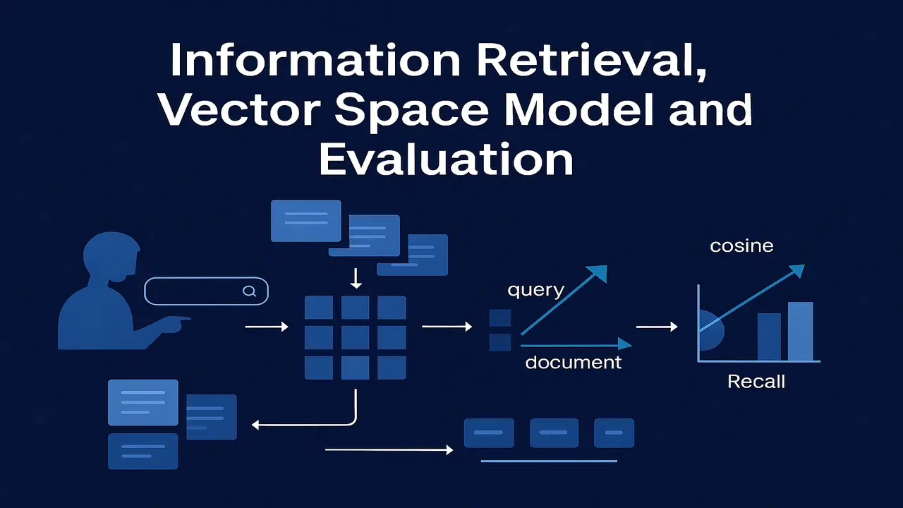
Vector space model. representing documents and queries

The next question is. how do we compare the content of a document with the content of a query

The vector space model answers this by representing both documents and queries as vectors of term weights in a high dimensional space.

Process overview.

Build a vocabulary of V terms from the corpus.
Represent each document as a V dimensional vector, where each component is a weight for a specific term.
Represent the query as another V dimensional vector built from the same vocabulary and weighting scheme.

If a document is about “information retrieval and vector space model”, it will have high weights for the terms “information”, “retrieval”, “vector”, “space” and “model”. A query containing “information retrieval vector space model” will produce a very similar pattern of high weights in those dimensions.

Documents and queries that are similar in topic and vocabulary end up as vectors pointing in similar directions in this space. Documents on unrelated topics will have very different vectors. This geometric view is powerful because similarity between documents and queries becomes a matter of vector similarity.

From bag-of-words and TF-IDF to vector representation

In earlier lectures, you built bag-of-words and TF-IDF representations for text classification. The same document term matrix is used by information retrieval systems. The difference lies in how we use the matrix.

For classification.

The document term matrix is the input to a classifier that learns decision boundaries between classes.

For retrieval.

The document term matrix directly defines the positions of documents in vector space, and each query is converted into the same space so we can compute similarity scores.

TF-IDF plays a crucial role here. Instead of counting how many times a word appears, TF-IDF gives higher weight to words that are frequent in a document but rare across the corpus, and lower weight to extremely common words that appear everywhere. This helps emphasise the terms that truly characterise a document’s content.

In vector space IR:

Term frequency captures local importance of a word in a document.
Inverse document frequency captures global discriminative power of that word across documents.
Their product forms TF-IDF weights that populate document and query vectors.

Because TF-IDF is already familiar from text classification, students can see IR as a new task built on the same representation.

Introduction to Information Retrieval – Online Book

Cosine similarity and ranking

Once documents and queries are represented as vectors, we need a numeric similarity measure. The standard choice in vector space IR is cosine similarity.

Given a query vector q and a document vector d, cosine similarity is defined as.

cosine(q, d) = (q · d) / (‖q‖ × ‖d‖)

The numerator is the dot product of the two vectors. the sum of elementwise products. The denominator is the product of the lengths of the two vectors. This normalisation ensures that the measure depends on the angle between the vectors rather than their absolute length.

Interpretation.

If a document contains the same important terms as the query with similar relative weights, the angle between q and d is small and cosine similarity is close to 1.
If the document uses very different vocabulary, the angle is large and cosine similarity approaches 0.

A basic vector space retrieval system works as follows.

Convert the user query to a TF-IDF vector q.
Use the inverted index to retrieve all documents that contain at least one query term.
For each candidate document with vector d, compute cosine(q, d).
Rank documents in descending order of similarity.
Present the top k documents as search results.

This produces a graded ranking rather than a simple yes or no “match”. Some documents are more similar to the query than others, and cosine similarity captures this intuition.

Lecture 10 – Text Classification with Bag-of-Words and TF-IDF in NLP

Evaluation. precision, recall and F1 in the IR context

In text classification, evaluation metrics were defined in terms of correct and incorrect label predictions. In information retrieval, we still use precision, recall and F1, but the focus shifts to relevance of retrieved documents.

Suppose for a given query.

R is the set of all relevant documents in the collection.
A is the set of documents retrieved by the system.

Then.

Precision = |A ∩ R| / |A|

This measures the fraction of retrieved documents that are actually relevant. High precision means users do not see many irrelevant results.

Recall = |A ∩ R| / |R|

This measures the fraction of relevant documents that were retrieved. High recall means the system is not missing many relevant results.

F1 score is the harmonic mean of precision and recall.

F1 = 2 × precision × recall / (precision + recall)

In ranked retrieval, we often consider only the top k results. For example, precision at 10 asks. among the first ten results, how many were relevant Precision, recall and F1 can be averaged over many queries to summarise system performance.

Practical observations.

High precision and low recall means the system is very selective and shows mostly correct results but hides many relevant documents.
High recall and low precision means users see most relevant documents, but they must sift through a lot of irrelevant ones.

Real systems often need to balance precision and recall depending on the application. Legal search might prioritise recall, while an e commerce site may prefer high precision on the first page of results.

Information retrieval, NLP and full search systems

It is useful to distinguish clearly between three layers of abstraction.

First, core information retrieval theory.

This includes vector space models, TF-IDF weighting, probabilistic models, BM25 scoring, inverted indexing and formal evaluation metrics. At this level, text is mostly treated as tokens and counts.

Second, Natural Language Processing enhancements.

Here, better tokenisation, stemming, lemmatisation, phrase detection, part-of-speech information and semantic similarity all help match queries and documents more intelligently. Query expansion with synonyms, handling of spelling errors and detection of phrases such as “machine learning” versus “machine” and “learning” separately are examples of NLP adding value to IR.

Third, full search engine implementation.

This is where scalable distributed indexing, freshness ranking, handling of duplicate pages, click-based learning-to-rank, personalisation and many other components come in. These systems may combine several scoring signals, including classical TF-IDF or BM25 scores and neural ranking models.

For this course, the priority is to master the core IR vector space model and its evaluation, while understanding how it connects to earlier lectures and to the wider ecosystem of search technologies.

Real Examples

You can place this section with a heading like “Real Applications of Information Retrieval”.

Course website search. Your NLP course website indexes all lecture pages and notes. When a student types “Hidden Markov Models and POS tagging”, the IR system scores lecture pages based on overlap in terms like “hidden”, “Markov”, “tagging” and “emission probabilities” and ranks the HMM lecture near the top.
Digital library search. A research portal indexes abstracts of NLP papers. A query such as “information retrieval vector space model evaluation” retrieves and ranks classic IR papers that discuss vector space ranking, TF-IDF and precision–recall trade-offs.
E commerce search. An online store indexes product titles and descriptions. A query “budget gaming laptop 16GB RAM” is matched against TF-IDF vectors of product descriptions. Products whose descriptions emphasise “gaming”, “16GB RAM” and “graphics card” get higher scores and appear earlier in results.
FAQ and help centre search. A company indexes its FAQ pages. When a user types “reset my password” or “cannot login account”, the IR system retrieves pages whose text is most similar to the query, even if the wording is not identical, improving self-service support.

These examples show how the same underlying vector space model and evaluation ideas can be applied in very different domains.

Step-by-Step Algorithm Explanation (Vector Space IR)

Step 1. Gather a corpus of documents to index.

Step 2. Apply preprocessing: lowercase, tokenize, optionally remove stopwords and apply stemming or lemmatization.

Step 3. Build a vocabulary of terms that appear in the corpus above a chosen frequency threshold.

Step 4. For each document, compute term frequencies and then TF-IDF weights for each vocabulary term. This gives you a document vector.

Step 5. Construct an inverted index mapping each term to the list of documents that contain it, optionally storing term frequencies or TF-IDF values in the postings.

Step 6. When a user submits a query, apply the same preprocessing and compute TF-IDF weights for the query terms using the same IDF values. This gives a query vector.

Step 7. Use the inverted index to retrieve the set of candidate documents that contain at least one query term.

Step 8. For each candidate document vector, compute cosine similarity between the query vector and the document vector.

Step 9. Rank candidate documents by decreasing cosine similarity and return the top k documents as the search results.

Step 10. If you have relevance judgments for queries, evaluate the system by computing precision, recall and F1 across those queries.

Code Examples (Python, scikit-learn)

A minimal example of vector space retrieval using TF-IDF and cosine similarity.

from sklearn.feature_extraction.text import TfidfVectorizer
from sklearn.metrics.pairwise import cosine_similarity
import numpy as np

# Example document collection (replace with your own corpus)
documents = [
    "Introduction to natural language processing and text preprocessing.",
    "Hidden Markov Models for part-of-speech tagging in NLP.",
    "Language modeling with n-grams, smoothing and backoff.",
    "Text classification using bag-of-words and TF-IDF features.",
    "Information retrieval with the vector space model and cosine similarity."
]

doc_ids = [f"doc_{i+1}" for i in range(len(documents))]

# Build TF-IDF document matrix
vectorizer = TfidfVectorizer(
    ngram_range=(1, 2),
    stop_words="english"
)
tfidf_matrix = vectorizer.fit_transform(documents)

def search(query, top_k=3):
    # Represent query in the same TF-IDF space
    query_vec = vectorizer.transform([query])

    # Compute cosine similarity between query and all documents
    scores = cosine_similarity(query_vec, tfidf_matrix)[0]

    # Get indices of highest scoring documents
    top_idx = np.argsort(scores)[::-1][:top_k]

    results = []
    for idx in top_idx:
        results.append({
            "doc_id": doc_ids[idx],
            "score": float(scores[idx]),
            "text": documents[idx]
        })
    return results

if __name__ == "__main__":
    query = "information retrieval vector space model"
    results = search(query, top_k=3)
    for r in results:
        print(f"{r['doc_id']} (score={r['score']:.3f}) -> {r['text']}")

Summary

Information retrieval provides the core technology behind search, and the vector space model is one of its most important frameworks. By representing documents and queries as TF-IDF vectors, computing cosine similarity and ranking results accordingly, we can build effective systems that connect users to relevant information in large text collections.

Indexing with inverted files makes retrieval efficient, while evaluation with precision, recall and F1 helps us understand how well a system performs and where it can be improved. These classical ideas continue to influence modern neural search systems, which still rely on vector representations and similarity measures, even though the vectors are now learned.

For any student of NLP, understanding information retrieval, the vector space model and evaluation metrics is essential preparation for designing search systems, experimenting with ranking models and moving towards advanced semantic or neural retrieval.

Next Lecture 12 – Information Extraction & Relation Extraction

Lecture 11 – Information Retrieval, Vector Space Model and Evaluation