Text classification is one of the most practical skills in Natural Language Processing. Whenever we automatically categorise emails into spam and non spam, label product reviews as positive or negative, or route support tickets to the right department, we are doing text classification.
This lecture focuses on classic text classification with bag-of-words and TF-IDF features combined with simple machine learning models. Naive Bayes and logistic regression are still strong baselines even in the era of transformers, and they are ideal for teaching the core ideas.
The goal of this lecture is to show how raw text is converted into a document term matrix, how features like n grams and TF-IDF are engineered, how simple classifiers are trained, and how to evaluate performance using accuracy, precision, recall and F1 score.
What is text classification in NLP
Text classification means assigning one or more labels to a piece of text. The labels can be topics, intents, sentiment categories, document types or any other categories relevant to the application.
Examples.
- Spam vs non spam for emails.
- Positive, negative, neutral for product reviews.
- News categories such as politics, sports, technology, entertainment.
- Internal labels like “billing issue”, “technical issue”, “general enquiry” for support tickets.
Formally, we have a set of documents and a set of classes. The aim is to learn a function from documents to classes that generalizes to new unseen text. For most undergraduate NLP courses, we focus on supervised classification, where each training document has a known label.
Bag-of-words representation
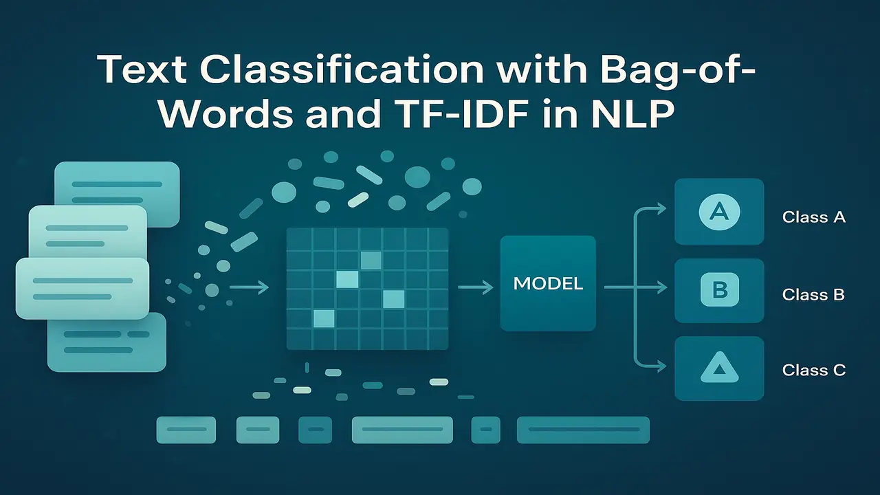
Raw text cannot be used directly by machine learning algorithms. We need a numeric representation. The simplest and still very effective representation is the bag-of-words model.
Bag-of-words makes three main assumptions.
- Word order is ignored inside each document.
- Only the presence, frequency or weighted importance of words matters.
- Each document is represented as a vector over the vocabulary.
To build a bag-of-words representation.
- Collect all training documents.
- Tokenise and normalise (lowercase, basic cleaning).
- Build a vocabulary of all unique tokens that appear frequently enough.
- For each document, count how many times each vocabulary word appears.
The result is a document term matrix. each row is a document, each column is a vocabulary word, and each cell contains a count or weight.
Even though bag-of-words ignores word order, it works surprisingly well for many classification tasks because topic and sentiment are often signalled by word usage. For example, documents containing “invoice”, “payment”, “due”, “overdue” are likely related to billing, regardless of exact word order.
Document term matrix and feature engineering
The document term matrix is the core data structure for classical text classification. However, pure unigram counts are not always enough. We can engineer additional features.
- N grams. Instead of using only single words, we also include bigrams or trigrams. For example, “machine learning” and “credit card” as features often carry more meaning than individual words “machine”, “learning”, “credit”, “card”.
- Binary vs count features. Some models work better with binary features that indicate presence or absence of a term rather than exact counts. For example, Bernoulli Naive Bayes uses binary indicators.
- Normalisation. Raw counts can be normalised by document length, or transformed with logarithms to reduce the impact of extremely frequent terms.
- TF-IDF weighting. Instead of raw counts we often use TF-IDF, which combines term frequency and inverse document frequency to highlight informative words.
The choice of features depends on the dataset size, domain and model. In many text classification tasks, unigram and bigram TF-IDF features with a linear classifier give strong performance.
TF-IDF for text classification
TF-IDF (Term Frequency × Inverse Document Frequency) is a weighting scheme that upgrades bag-of-words from simple counts to more informative numeric features.
- Term frequency captures how many times a term appears in a document.
- Inverse document frequency downweights terms that appear in many documents, because such terms are not helpful for distinguishing classes.
A common variant is.
- tf(t, d) = 1 + log(count of t in d) if count > 0, otherwise 0.
- idf(t) = log(N / df(t)) where N is number of documents and df(t) is number of documents containing t.
- TF-IDF weight w(t, d) = tf(t, d) × idf(t).
In a spam classifier, words like “money”, “free”, “offer”, “win” may receive high TF-IDF weights in spam documents, whereas very common words like “the” and “and” are downweighted. Models built on TF-IDF features often outperform models using raw counts, especially when the vocabulary is large.
Simple classifiers. Naive Bayes and logistic regression
Once we have a document term matrix, we can use standard machine learning algorithms. Two of the most common choices are Naive Bayes and logistic regression.
Naive Bayes
Naive Bayes is a probabilistic classifier that assumes features (words) are conditionally independent given the class. Despite this strong assumption, it works well for text because high dimensional sparse features and word frequency patterns fit the model reasonably.
In the multinomial Naive Bayes variant.
- For each class c, we estimate the probability of each word given that class, P(word | c), using counts with smoothing.
- For a new document, we compute the posterior probability of each class using Bayes’ rule and the product of word likelihoods.
Advantages:
- Very fast to train and predict.
- Works well on small to medium sized datasets.
- Particularly good when features are counts or TF features.
Limitations:
- Independence assumption is unrealistic.
- Decision boundaries are often less flexible than discriminative models.
Logistic regression
Logistic regression is a linear discriminative classifier. Instead of modelling P(words | class), it models P(class | features) directly.
- Each word (or n-gram) gets a learned weight for each class.
- Features are usually TF-IDF or normalised counts.
- The model finds weights that separate classes by maximising the likelihood or minimising cross entropy loss.
Advantages.
- Typically higher accuracy than Naive Bayes when training data is sufficient.
- Works very well with high dimensional sparse features.
- Coefficients are interpretable. positive weights indicate features that support a class.
Limitations.
- Training is slower than Naive Bayes for very large datasets, but still efficient with modern solvers.
For many undergraduate projects, multinomial Naive Bayes and logistic regression form the main baseline models for text classification.
Typical text classification pipeline
Putting everything together, a standard pipeline for text classification with bag-of-words and TF-IDF looks like this.
- Data collection. gather documents and their labels, for example product reviews with ratings.
- Train test split. separate a portion of data for evaluation.
- Preprocessing. lowercase, tokenise, optionally remove stopwords or apply lemmatisation.
- Feature extraction.
- Build a vocabulary from the training set.
- Compute TF-IDF features using unigrams and possibly bigrams.
- Model training. train a classifier such as multinomial Naive Bayes or logistic regression on the training features and labels.
- Model evaluation. evaluate on the test set and compute accuracy, precision, recall and F1.
- Error analysis. inspect misclassified examples to understand patterns and improve preprocessing or features.
This pipeline is simple yet forms the basis of many production systems, especially where data is not extremely large or real time constraints are moderate.
Real world style examples
A few practical scenarios where bag-of-words and TF-IDF text classification are used.
- Email spam filtering. a provider trains a classifier on millions of labelled emails. Words like “lottery”, “prize”, “urgent response”, “winner” get high weights for the spam class, while normal conversational vocabulary points to ham.
- Product review sentiment. an e commerce site uses TF-IDF features and logistic regression to predict sentiment from user reviews. Terms like “excellent”, “highly recommend”, “totally worth it” support the positive class, while “waste of money”, “poor quality”, “broke after a week” support negative.
- Support ticket routing. a company automatically routes incoming tickets to “billing”, “technical support”, “sales enquiry”. Bag-of-words features highlight domain specific terms. “invoice”, “payment”, “refund” → billing. “error”, “crash”, “update” → technical. “pricing”, “quotation”, “discount” → sales.
- News topic classification. a news aggregator uses text classification to cluster articles into sports, politics, technology and entertainment, feeding them into topic specific pages.
These systems often started historically with bag-of-words models and later added more advanced approaches, but classic models remain strong baselines and are still used when interpretability and simplicity are valued.
- Step-by-step algorithm explanation (bag-of-words + logistic regression)
A clear step-by-step algorithm you can highlight in a separate box:
- Input. labelled documents D = {(d₁, y₁), …, (dₙ, yₙ)}.
- Preprocess each document dᵢ. lowercase, tokenise, optionally remove stopwords.
- Build a vocabulary V of all terms that appear at least k times in the training set.
- Use TF-IDF to convert each document into a feature vector xᵢ ∈ ℝ^|V|.
- Split data into training and test sets.
- Train a logistic regression classifier on training vectors (xᵢ, yᵢ).
- For a new document, convert it to a TF-IDF vector using the same vocabulary and IDF values.
- Use the trained model to predict its class label and class probabilities.
- Evaluate using accuracy, precision, recall and F1 on the held out test set.
Code examples (Python, scikit-learn)
from sklearn.model_selection import train_test_split
from sklearn.feature_extraction.text import TfidfVectorizer
from sklearn.linear_model import LogisticRegression
from sklearn.metrics import classification_report, accuracy_score

# Example documents and labels (replace with real dataset)
texts = [
    "Great battery life and excellent camera, highly recommend this phone",
    "Terrible sound quality, very disappointed with these headphones",
    "The laptop is okay for basic tasks, nothing special",
    "Best purchase I made this year, amazing performance",
    "Complete waste of money, stopped working after a week"
]
labels = ["positive", "negative", "neutral", "positive", "negative"]

# Train-test split
X_train, X_test, y_train, y_test = train_test_split(
    texts, labels, test_size=0.4, random_state=42
)

# TF-IDF vectoriser with unigrams and bigrams
vectorizer = TfidfVectorizer(
    ngram_range=(1, 2),
    max_features=5000,
    min_df=1,
    stop_words="english"
)
X_train_vec = vectorizer.fit_transform(X_train)
X_test_vec = vectorizer.transform(X_test)

# Logistic regression classifier
clf = LogisticRegression(max_iter=1000)
clf.fit(X_train_vec, y_train)

# Evaluation
y_pred = clf.predict(X_test_vec)
print("Accuracy:", accuracy_score(y_test, y_pred))
print(classification_report(y_test, y_pred))

# Predict on new examples
new_texts = [
    "The service was slow and the food was cold",
    "Fast delivery and great packaging, very happy"
]
new_vec = vectorizer.transform(new_texts)
print(clf.predict(new_vec))
For a second lab, you can replace logistic regression with multinomial Naive Bayes and compare performance.
Summary
Text classification with bag-of-words and TF-IDF is one of the most important foundations in Natural Language Processing. By converting documents into vectors of term weights and training simple yet powerful classifiers such as Naive Bayes and logistic regression, we can build systems for spam filtering, sentiment analysis, topic categorisation and many other real applications.
Although modern deep learning models use embeddings and transformers, classic bag-of-words pipelines remain valuable. They are easy to implement, fast to train and surprisingly strong baselines. More importantly, they help students understand the relationship between vocabulary, document statistics, feature engineering and evaluation metrics, which carries over directly to more advanced models.
Next. Lecture 11 – Information Retrieval & Vector Space Model
People also ask:
Text classification is the task of automatically assigning predefined labels to text, such as spam vs non spam, sentiment categories or topic labels. It converts raw text into numeric features and uses machine learning models to predict the most likely class for each document.
The bag-of-words model represents each document as a vector of word frequencies or weights, ignoring word order. Each dimension corresponds to a vocabulary term and the value shows how often or how strongly that term occurs in the document. This numeric representation is then used as input to classifiers such as Naive Bayes or logistic regression.
TF-IDF reduces the impact of very common words that appear in almost every document and emphasizes terms that are frequent in a specific document but rare overall. This makes features more informative and often improves classification accuracy compared to using raw counts.
Common algorithms include multinomial Naive Bayes, logistic regression, linear Support Vector Machines and sometimes decision trees or random forests. For high dimensional sparse text data, linear models such as Naive Bayes, logistic regression and linear SVMs are usually preferred.
Models are usually evaluated on a held out test set using metrics such as accuracy, precision, recall and F1 score. Confusion matrices help you see which classes are often confused, and macro averaged F1 is useful when classes are imbalanced.