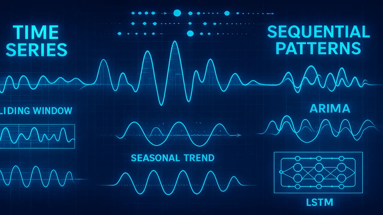
Lecture 14 - Time Series Data Mining & Sequential Pattern Analysis

Lecture 14 explains time series data mining, sequential pattern algorithms, forecasting models (ARIMA, LSTM), preprocessing, similarity measures, anomaly detection, and real-world applications in finance, healthcare, IoT, and cybersecurity.

Time-series data is everywhere stock markets, weather sensors, medical signals, website traffic, electricity consumption, and network logs. Unlike static datasets, time-series data captures values across time, meaning patterns, trends, seasonal behaviors, and anomalies can reveal powerful insights.

This lecture teaches how to prepare, analyze, model, and mine time-series and sequential patterns for real-world AI applications.

Introduction to Time-Series Mining

What Is Time-Series Data?

Time-series data is any information recorded at regular time intervals.

Examples:

Daily temperature
Hourly electricity usage
Minute-by-minute heart rate
Stock prices every second

Why Time-Series Matters in Data Mining

Because the order of data points matters.

Time influences:

Trends
Cycles
Correlations
Patterns
Predictions

Components of Time-Series

Trend

Long-term increase or decrease over years.

Seasonality

Repeating patterns (daily, monthly, yearly).

Cyclic Behavior

Irregular economic cycles (booms, recessions).

Noise

Random fluctuations caused by unpredictable events.

Time-Series Preprocessing

Preparing time-series data is more complex than normal datasets.

Handling Missing Time Steps

Methods:

Forward fill
Interpolation
Model-based imputation

Example (Python-style):

df = df.asfreq('D').interpolate()

Smoothing & Filtering

Used to remove noise.

Methods:

Moving average
Exponential smoothing
Low-pass filters

Stationarity

For many forecasting models (ARIMA), data must be stationary.

Check with:

ADF test
Rolling mean

Fix using:

Differencing
Log transforms
Detrending

Normalization & Scaling

Common techniques:

Min-Max Scaling
Z-score Standardization

Essential for neural networks.

Deep Learning Course

Time-Series Feature Extraction

Statistical Features

Mean
Variance
Skewness
Kurtosis

Rolling Windows

Extract features over sliding windows.

Example:

df['mean_7'] = df['value'].rolling(7).mean()

Fourier & Wavelet Transforms

Used to analyze frequency patterns.

Applications:

Speech mining
ECG signals
Machinery vibration analysis

Sequential Pattern Mining

Sequential Pattern Mining discovers frequent sequences in ordered datasets.

GSP Algorithm (Generalized Sequential Patterns)

Steps:

Generate candidate sequences
Count support
Keep frequent sequences
Repeat

PrefixSpan Algorithm

Avoids candidate generation.
Build sequences by growing prefixes.

SPADE Algorithm

Uses vertical data format for scalability.

Time-Series Similarity Measures

Euclidean Distance

Works for equal-length, aligned sequences.

Dynamic Time Warping (DTW)

Handles sequences with different speeds.

Used for:

Speech
Handwriting
Wearables

TensorFlow Time-Series Tutorials

Correlation-Based Similarity

Measures how two sequences move together.

Time-Series Classification

Distance-Based Methods

1-NN + DTW
Shapelet transforms

Feature-Based Methods

Extract features → use ML models.

Deep Learning Approaches

CNN on time-series images
RNN/LSTM
Transformer models

Time-Series Forecasting Models

AR, MA & ARMA

Classical statistical models.

ARIMA & SARIMA

ARIMA handles:

Trends
Autocorrelation
Noise

SARIMA adds:

Seasonality

Prophet Model (by Meta/Facebook)

Great for:

Missing data
Holidays
Seasonality

LSTM & GRU Models

Best for:

Long temporal patterns
Irregular data
Multi-step forecasting

Diagram:

Input Sequence → LSTM Cells → Dense → Forecast

Lecture 13 – Deep Learning for Data Mining Foundations, Architectures & Applications

Anomaly Detection in Time-Series

Statistical Thresholding

Find outliers based on:

Z-score
Confidence intervals
IQR

Isolation-Based Methods

Isolation forest isolates anomalies easily.

Autoencoder Detection

Autoencoders produce high reconstruction error for anomalies.

Real-World Applications

Finance

Stock market prediction
Fraud detection
Risk scoring

Healthcare

ECG/EEG analysis
Patient monitoring
Disease detection

IoT & Sensor Data

Smart home automation
Industrial machinery
Environmental monitoring

Cybersecurity

Botnet detection
Intrusion detection
Network traffic anomalies

Summary

Lecture 14 explored the complete world of time-series data mining: data preparation, rolling windows, sequential patterns, similarity measures, forecasting models including ARIMA and LSTM, anomaly detection, and real-world applications. Students now understand how to mine temporal data and build forecasting systems used across finance, medicine, IoT, and cyber analytics.