Lectures 4 – Adaline and Delta Rule in Neural Networks Explained with Gradient Descent

Learn Adaline and Delta Rule in neural networks in depth. Understand gradient descent, Mean Squared Error, weight updates, learning rate, and the difference between Adaline and Perceptron.

Introduction

Artificial Neural Networks are inspired by the way the human brain processes information. In the early development of neural network models, researchers introduced simple computational neurons to solve classification and prediction problems. One of the earliest and most important models in this evolution is Adaline, which stands for Adaptive Linear Neuron.

Adaline is an important topic because it introduced a more mathematically sound learning approach than the Perceptron. While the Perceptron can only learn by correcting classification errors after thresholding, Adaline learns by reducing the difference between the predicted output and the actual target value. This difference is measured using an error function, and the model updates its weights through a method known as the Delta Rule.

The Delta Rule is closely connected with Gradient Descent, which later became one of the most fundamental optimization techniques in machine learning and deep learning. Understanding Adaline and the Delta Rule helps students build a strong foundation before studying backpropagation, multilayer perceptrons, and deep neural networks.

This lecture explains the concept of Adaline in detail, how it works, how the Delta Rule updates weights, why gradient descent is important, and how Adaline differs from the Perceptron.

What Is Adaline?

Adaline, or Adaptive Linear Neuron, is a single-layer neural network model developed to improve learning performance in classification tasks. Structurally, it looks similar to a Perceptron because both models take input values, multiply them with weights, add a bias, and produce an output. However, the key difference is not only in the final output but in the way learning takes place.

Adaline uses a linear activation function during learning. Instead of applying a hard threshold immediately and then deciding whether the output is right or wrong, it first works with the raw weighted sum. The error is computed using this continuous output, and then the weights are adjusted to reduce this error.

This makes Adaline much more suitable for optimization because the error function becomes smooth and differentiable. A smooth error function allows the use of calculus-based techniques like gradient descent, which helps the model move gradually toward better solutions.

In simple words, Adaline does not just ask, “Was the answer right or wrong?” It asks, “How far was my answer from the correct answer?” That small change makes the learning process more powerful and more scientific.

Why Adaline Was Introduced

The Perceptron was an important early model, but it had several limitations. It could learn only linearly separable problems, and its learning rule was based on whether the final classified output was correct or incorrect. This means the Perceptron did not consider the magnitude of the error. A prediction that was slightly wrong and a prediction that was very wrong could both be treated in the same way.

Adaline improved this situation by introducing an error-minimization approach. Instead of using only the thresholded final output, it used the raw linear output to calculate the error. This allowed more informative weight updates.

The introduction of Adaline was significant because it moved neural network learning from a simple correction mechanism to a numerical optimization problem. That idea later became central in training modern machine learning models.

Basic Architecture of Adaline

The architecture of Adaline is simple and easy to understand. It consists of the following main parts:

Input Layer

The input layer contains the features or values fed into the model. These can be represented as:

• x1
• x2
• x3
• and so on

Each input corresponds to one feature of the data.

Weights

Each input has an associated weight:

• w1
• w2
• w3
• and so on

Weights determine how important each input is in producing the output.

Bias

A bias term is added to shift the decision boundary. It helps the model fit data more flexibly.

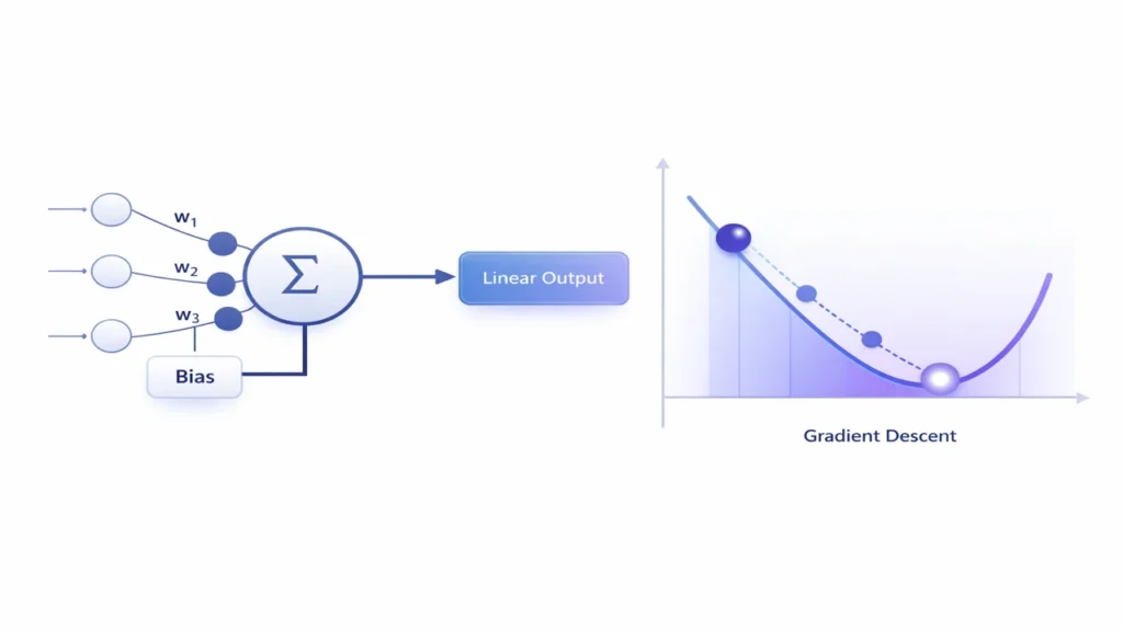
Summation Unit

The inputs are multiplied by their corresponding weights, and then all products are added together with the bias.

So the net input is:

z = w1x1 + w2x2 + w3x3 + … + b

Linear Activation

Adaline uses a linear activation during learning. That means the output is simply the weighted sum:

y = z

This continuous value is then used to compute the error.

Threshold for Final Classification

In classification tasks, a threshold can be applied later to convert the continuous output into a class label, but this thresholded value is not used for learning. Learning is based on the raw linear output.

Mathematical Model of Adaline

The mathematical model of Adaline can be written as follows.

Let the input vector be:

x = [x1, x2, x3, …, xn]

Let the weight vector be:

w = [w1, w2, w3, …, wn]

Then the net input is:

z = w.x + b

where w.x represents the dot product of weights and inputs.

The output of Adaline is:

y = z

If this is used for binary classification, then after learning we may apply a threshold such as:

• if y ≥ 0, class = 1
• if y < 0, class = -1

However, during training, the model does not use this thresholded class output for calculating error. Instead, it compares the actual target value directly with the raw output y.

This is one of the most important points in understanding Adaline.

Lectures 3 – Perceptron Learning Model Explained

How Adaline Works Step by Step

The working of Adaline can be broken into a series of simple steps.

Step 1: Take Input Values

The model receives a set of input features from the training data.

Step 2: Multiply by Weights

Each input is multiplied by its corresponding weight.

Step 3: Add Bias

The weighted values are summed and bias is added.

Step 4: Produce Linear Output

The model produces a continuous output value.

Step 5: Compare with Target

The predicted output is compared with the actual target output.

Step 6: Calculate Error

The difference between target and predicted output is used to compute error.

Step 7: Update Weights

The weights are adjusted to reduce the error.

Step 8: Repeat

This process continues for many training examples over multiple iterations until the error becomes small enough.

This repeated adjustment of weights is what allows the network to learn.

The Need for an Error Function

A model cannot improve unless it knows how bad its predictions are. This is why an error function is needed.

In Adaline, the most commonly used error function is the Mean Squared Error (MSE). The idea is simple: take the difference between actual and predicted values, square it, and average it across all training examples.

The formula is:

MSE = (1/n) Σ (t – y)^2

where:

• n = number of training samples
• t = target value
• y = predicted output

Squaring serves two purposes:

First, it removes negative signs, so positive and negative errors do not cancel each other out.

Second, it penalizes large errors more heavily than small errors.

This makes MSE a useful and smooth error function for optimization.

Why Mean Squared Error Is Important in Adaline

Mean Squared Error is one of the central ideas in Adaline. It is important for several reasons.

It Measures Magnitude of Error

Unlike simple right-or-wrong checking, MSE tells us how far the prediction is from the actual target.

It Is Differentiable

Because MSE is smooth, we can calculate its gradient. This is essential for gradient descent.

It Supports Systematic Learning

Instead of random updates or basic correction rules, MSE allows the network to update weights in a mathematically guided way.

It Leads to Better Convergence

A differentiable error surface makes it easier to move gradually toward a minimum error solution.

This is why Adaline is considered a major step forward from the Perceptron.

What Is the Delta Rule?

The Delta Rule is the learning rule used in Adaline to update weights so that the error decreases over time.

The word “delta” means change. In this case, it refers to the change required in weights to make the network’s output closer to the target output.

The Delta Rule adjusts each weight based on three things:

• the input value
• the prediction error
• the learning rate

The weight update formula is:

w(new) = w(old) + η (t – y) x

where:

• η is the learning rate
• t is the target output
• y is the predicted output
• x is the input associated with that weight

Similarly, the bias can be updated as:

b(new) = b(old) + η (t – y)

This rule says that if the error is large, the weight change should be larger. If the input value is large, the related weight should also be adjusted more strongly. If the learning rate is small, learning becomes slower and safer.

Understanding the Delta Rule Intuitively

To understand the Delta Rule intuitively, imagine that the model’s output is lower than the correct answer. In that case, the error term (t - y) is positive. The model will increase the relevant weights so the next prediction becomes larger.

If the model’s output is greater than the correct answer, the error term becomes negative. Then the model reduces the relevant weights to bring the output down.

So the Delta Rule is essentially a controlled correction mechanism that pushes the output toward the target in small steps.

This gradual improvement is much more stable than making abrupt yes-or-no corrections.

What Is Gradient Descent?

Gradient Descent is an optimization method used to minimize the error function. It is one of the most important concepts in machine learning and deep learning.

To understand Gradient Descent, imagine you are standing on a hill in the fog and want to reach the lowest point in the valley. You cannot see the whole landscape, but you can feel the slope beneath your feet. So you take a small step in the direction that goes downward. Then again you check the slope and take another step downward. Repeating this eventually brings you close to the lowest point.

In the same way, Gradient Descent looks at the direction in which the error decreases most rapidly and updates the weights in that direction.

In Adaline, the Delta Rule is derived from Gradient Descent. That means Adaline learns by moving step by step toward lower Mean Squared Error.

Relationship Between Delta Rule and Gradient Descent

The Delta Rule is not separate from Gradient Descent. It is actually an application of Gradient Descent to the Adaline model.

The error function depends on the weights. If we calculate the derivative of the error with respect to each weight, we learn how the error changes when that weight changes.

The gradient tells us the direction of greatest increase in error. Since we want to reduce error, we move in the opposite direction of the gradient.

That is why the general gradient descent update is:

w(new) = w(old) – η (∂E/∂w)

For Adaline, when this derivative is worked out using the MSE error function, it leads to the Delta Rule form.

So the Delta Rule is simply the practical weight-update rule that results from minimizing MSE using Gradient Descent.

Learning Rate and Its Role in Training

The learning rate, usually represented by η, controls the size of each weight update.

It is one of the most important hyperparameters in neural network training.

If Learning Rate Is Too Small

The model learns very slowly. Training may take too much time, and convergence becomes inefficient.

If Learning Rate Is Too Large

The model may overshoot the minimum error point. Instead of gradually reaching the best solution, it may jump around and fail to converge.

If Learning Rate Is Properly Chosen

The model learns at a good speed and gradually reduces error in a stable way.

You can think of the learning rate like the step size while walking downhill. Very small steps are safe but slow. Very large steps are fast but risky. A balanced step size is best.

Adaline Training Process in Detail

The complete training process of Adaline generally follows these steps:

1. Initialize Weights and Bias

Start with small random values.

2. Present a Training Example

Feed one input vector into the network.

3. Compute Net Input

Calculate the weighted sum plus bias.

4. Compute Output

Because Adaline uses a linear activation, the output is the same as the net input.

5. Calculate Error

Find the difference between target and output.

6. Update Weights Using Delta Rule

Adjust each weight to reduce error.

7. Update Bias

Adjust bias as well.

8. Repeat for All Training Samples

This completes one epoch.

9. Continue for Multiple Epochs

Training continues until the total error becomes sufficiently low or the maximum number of epochs is reached.

This iterative process gradually improves the model’s ability to make predictions.

Simple Numerical Example of Adaline and Delta Rule

Let us take a simple example.

Assume:

• input x = 2
• target t = 1
• initial weight w = 0.5
• bias b = 0
• learning rate η = 0.1

Step 1: Compute Output

Since Adaline uses linear activation:

y = wx + b = (0.5)(2) + 0 = 1

Step 2: Calculate Error

error = t – y = 1 – 1 = 0

In this case, there is no error, so no weight update is needed.

Now suppose initial weight was:

w = 0.2

Then:

y = (0.2)(2) = 0.4

error = 1 – 0.4 = 0.6

Now update the weight:

w(new) = 0.2 + 0.1(0.6)(2)
w(new) = 0.2 + 0.12 = 0.32

Now the new weight is 0.32, which will produce a higher output next time and move the model closer to the target.

This simple example shows how the Delta Rule gradually adjusts weights toward better predictions.

Difference Between Adaline and Perceptron

This is one of the most important exam and conceptual questions.

Although Adaline and Perceptron appear similar in structure, they differ strongly in learning behavior.

1. Output Used for Learning

• Perceptron: Uses thresholded output for learning
• Adaline: Uses raw linear output for learning

2. Error Measurement

• Perceptron: Focuses on misclassification only
• Adaline: Uses Mean Squared Error

3. Learning Method

• Perceptron: Weight correction based on classification result
• Adaline: Weight update based on Delta Rule and Gradient Descent

4. Optimization

• Perceptron: No smooth error surface
• Adaline: Smooth differentiable error surface

5. Mathematical Strength

• Perceptron: Simpler but less refined
• Adaline: More mathematically grounded

In short, the Perceptron is an early classifier, while Adaline is an early optimization-based neural model.

Why Adaline Is Important for Deep Learning

Adaline may be an old and simple model, but its ideas are extremely important in modern deep learning.

Foundation of Error Minimization

Adaline introduced the concept of learning by minimizing an explicit error function.

Basis for Gradient-Based Learning

Its Delta Rule is an early form of gradient-based optimization.

Preparation for Backpropagation

Backpropagation in multilayer networks also depends on derivatives and gradient descent. Without understanding Adaline, it becomes harder to understand how deep networks learn.

Strong Conceptual Bridge

Adaline acts as a bridge between simple neural units and advanced trainable networks.

So even though modern systems are much more complex, the core idea is still similar: compute output, measure error, calculate gradient, and update weights.

Strengths of Adaline

Adaline has several educational and practical strengths.

Simple to Understand

Its structure is straightforward, making it ideal for beginners in neural networks.

Mathematically Meaningful

It introduces students to optimization, error functions, and iterative learning.

Better Than Basic Perceptron in Learning Logic

It uses actual prediction error rather than only thresholded classification error.

Good Foundation for Advanced Topics

Concepts such as MSE, gradient descent, and learning rate all prepare students for deep learning.

Limitations of Adaline

Like every model, Adaline also has limitations.

Limited to Simple Problems

Adaline is a single-layer model, so it cannot solve highly complex or non-linear problems on its own.

Linear Nature

Because it is based on a linear unit, its representation power is limited compared with deep networks.

Sensitive to Hyperparameters

Improper learning rate can make training slow or unstable.

Outdated for Large Modern Tasks

Today, more advanced models like multilayer perceptrons, CNNs, and RNNs are used for real-world deep learning tasks.

Still, Adaline remains very valuable for conceptual learning.

Real-World Relevance of Adaline Concepts

Even if Adaline itself is not widely used in modern large-scale applications, the concepts behind it are everywhere.

In Machine Learning

Loss functions, optimization, and gradient-based training are used in regression, classification, and neural networks.

In Deep Learning

Training of deep neural networks still depends on minimizing error with gradient-based methods.

In Signal Processing

Adaline historically played an important role in adaptive filtering and signal-related tasks.

In Education

Adaline is one of the best models to teach how a network actually learns.

So studying Adaline is not about memorizing an old model. It is about understanding the roots of modern AI learning systems.

Frequently Asked Questions

Conclusion

Adaline and the Delta Rule represent a major milestone in the development of artificial neural networks. This model showed that learning could be treated as a mathematical optimization problem rather than just a yes-or-no correction process. By introducing Mean Squared Error and Gradient Descent-based weight updates, Adaline laid the groundwork for many of the methods that power modern deep learning today.

For students of Artificial Neural Networks and Deep Learning, this topic is not just historical. It is foundational. Once you understand how Adaline learns, you can more easily understand how deeper and more complex neural networks are trained.

Adaline teaches one of the most important lessons in AI: a model becomes intelligent not just by making predictions, but by learning systematically from its mistakes.