Learn activation functions in neural networks in depth. Understand Sigmoid, ReLU, Tanh, Softmax, vanishing gradient, and their role in deep learning.

Introduction

Artificial Neural Networks are designed to simulate how the human brain processes information. Each neuron receives inputs, processes them, and produces an output. However, if neurons only performed simple linear calculations, neural networks would fail to solve real-world problems.

This is where activation functions play a critical role.

Activation functions introduce non-linearity, enabling neural networks to learn complex relationships in data. Without them, even a deep neural network would behave like a simple linear regression model.

In this lecture, we will deeply explore:

• What activation functions are
• Why they are necessary
• Types of activation functions
• Mathematical behavior
• Problems like vanishing gradient
• Real-world applications

What is an Activation Function?

An activation function is a mathematical function applied to the output of a neuron after the weighted sum is calculated.

Let’s define the neuron mathematically:

• Inputs: x₁, x₂, x₃
• Weights: w₁, w₂, w₃
• Bias: b

The neuron computes:

z = w₁x₁ + w₂x₂ + w₃x₃ + b

Then activation function is applied:

Output = f(z)

Here, f(z) is the activation function.

Why Do We Need Activation Functions?

To understand this, we must first understand the limitation of linear models.

Case 1: Without Activation Function

If no activation function is used:

Output = z = wx + b

Now imagine stacking multiple layers:

Layer 1 → Layer 2 → Layer 3

Even then, mathematically:

The entire network becomes linear combination of inputs

Result:

• No matter how deep the network is
• It behaves like one single linear model

Case 2: With Activation Function

Now introduce a non-linear function:

Output = f(wx + b)

Now each layer transforms data non-linearly.

Result:

• Network can learn:
  • Images
  • Speech
  • Language
  • Complex patterns

This is why activation functions are the heart of deep learning

Lectures 4 – Adaline and Delta Rule in Neural Networks Explained with Gradient Descent

Understanding Non-Linearity

Real-world data is rarely linear.

Example:

• Image classification → Not linear
• Face detection → Not linear
• Stock prediction → Not linear

Without non-linearity:
Model cannot separate complex patterns

Activation functions allow the model to:

• Bend decision boundaries
• Learn curves instead of straight lines

Types of Activation Functions

1. Step Function

Definition:

It outputs either 0 or 1 based on threshold.

Behavior:

• If input ≥ 0 → Output = 1
• If input < 0 → Output = 0

Use:

• Early Perceptron models

Limitations:

• Not differentiable
• Cannot be used in gradient-based learning
• Very rigid

This is why modern neural networks don’t use it

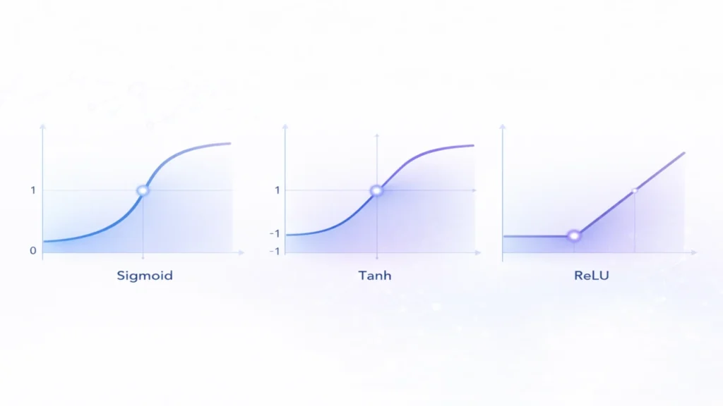
2. Sigmoid Function

$f(x) = \frac{1}{1 + e^{-x}}$

Characteristics:

• Output range: 0 to 1
• Smooth curve
• S-shaped

Advantages:

• Good for probability interpretation
• Used in binary classification

Problems:

1. Vanishing Gradient

For very large or very small values:

• Gradient becomes near zero
• Learning slows down

2. Not Zero-Centered

Outputs always positive → affects optimization

3. Tanh Function

$f(x) = \tanh(x)$

Characteristics:

• Output range: -1 to +1
• Zero-centered

Advantages:

• Better than sigmoid
• Faster convergence

Problems:

• Still suffers from vanishing gradient

4. ReLU (Rectified Linear Unit)

$f(x) = \max(0, x)$f(x)=max(0,x)

Behavior:

• If x < 0 → 0
• If x ≥ 0 → x

Advantages:

1. Computational Efficiency

• Simple operation → very fast

2. Avoids Vanishing Gradient

• Gradient = 1 for positive values

3. Sparse Activation

• Some neurons inactive → efficient

Problem: Dead Neurons

If neuron outputs 0 always:
It stops learning

5. Leaky ReLU

Definition:

Fixes dead neuron problem

• If x > 0 → x
• If x < 0 → small value (e.g., 0.01x)

Advantage:

• Keeps neurons alive

6. Softmax Function

Used in multi-class classification

Behavior:

Converts outputs into probabilities:

• All outputs sum to 1
• Each value between 0 and 1

Example:

Output:

• Cat: 0.7
• Dog: 0.2
• Car: 0.1

Use Cases:

• Image classification
• NLP classification

Vanishing Gradient Problem

This is one of the most important concepts in deep learning.

What Happens?

In deep networks:

• Gradients pass through many layers
• With sigmoid/tanh → gradients shrink

Eventually:

• Gradient ≈ 0
• Learning stops

Why It’s Dangerous?

• Early layers stop learning
• Model becomes ineffective

Solutions:

• Use ReLU
• Use better initialization
• Use batch normalization

Comparison of Activation Functions

Function	Range	Speed	Problem
Step	0/1	Fast	Not usable
Sigmoid	0–1	Slow	Vanishing gradient
Tanh	-1 to 1	Medium	Vanishing gradient
ReLU	0–∞	Fast	Dead neurons
Leaky ReLU	-∞ to ∞	Fast	Slight complexity
Softmax	0–1	Medium	Expensive

Real-World Applications

Computer Vision

• CNN uses ReLU

NLP

• Softmax for classification

Binary Classification

• Sigmoid

Frequently Asked Questions

Conclusion

Activation functions transform neural networks from simple linear systems into powerful deep learning models. Without them, modern AI would not exist. Understanding activation functions is essential before moving to backpropagation and deep architectures.